Annex J(Clauses 5.1.12 and 5.3.3.5.3)

NBC 2016 (SP 7:2016) Volume 1

2016 · PDF page 532

Hover any section to copy its link or text, ask Copilot about it, or bookmark it.

Simplified Procedure for Evaluation of Liquefaction Potential

J-1 Due to the difficulties in obtaining and testing undisturbed representative samples from potentially liquefiable sites, in-situ testing is the approach preferred widely for evaluating the liquefaction potential of a soil deposit. Liquefaction potential assessment procedures involving both the SPT and CPT are widely used in practice. The most common procedure used in engineering practice for the assessment of liquefaction potential of sands and silts is the simplified procedure. The procedure may be used with either standard penetration test (SPT) blow count or cone penetration test (CPT) tip resistance or shear wave velocity $V_{s}$ measured within the deposit as described below:

Step 1 — The subsurface data used to assess liquefaction susceptibility should include the location of the water table, either SPT blow count N or tip resistance $q_{c}$ of a CPT cone or shear wave velocity $V_{s}$ , unit weight, and fines content of the soil (percent by weight passing the IS Sieve No. 75μ).

Step 2 — Evaluate total vertical overburden stress $\sigma_{vo}$ and effective vertical overburden stress $\sigma'_{vo}$ at different depths for all potentially liquefiable layers within the deposit.

Step 3 — Evaluate stress reduction factor $r_{\mathrm{d}}$ using:

r _ {\mathrm{d}} = \left\{ \begin{array}{l l} 1 - 0. 0 0 7 6 5 z & 0 < z \leq 9. 1 5 \mathrm{m} \\ 1. 1 7 4 - 0. 0 2 6 7 z & 9. 1 5 < z \leq 2 3. 0 \mathrm{m} \end{array} \right.

where $z$ is the depth (in metre) below the ground surface.

Step 4 — Calculate cyclic stress ratio CSR induced by the earthquake using:

C S R = 0. 6 5 \left(\frac {a _ {\max}}{\mathrm{g}}\right) \left(\frac {\sigma_ {\mathrm{vo}}}{\sigma_ {\mathrm{vo}} ^ {\prime}}\right) r _ {\mathrm{d}},

where

$a_{\mathrm{max}} =$ peak ground acceleration (PGA) preferably in terms of $\mathrm{g}$ ,

$g =$ acceleration due to gravity, and

$r_{\mathrm{d}} =$ stress reduction factor.

If value of PGA is not available, the ratio $(a_{\mathrm{max}} / \mathrm{g})$ may be taken equal to seismic zone factor $Z$ (as per Table 42).

Step 5 — Obtain cyclic resistance ratio CRR by correcting standard cyclic resistance ratio $CRR_{7.5}$ for earthquake magnitude, high overburden stress level and high initial static shear stress using:

C R R = C R R _ {7, 5} (M S F) K _ {\sigma} K _ {a},

PART 6 STRUCTURAL DESIGN — SECTION 1 LOADS, FORCES AND EFFECTS

where

$CRR_{7.5}=$ standard cyclic resistance ratio for a 7.5 magnitude earthquake obtained using values of SPT or CPT or shear wave velocity (as per Step 6), and

MSF = magnitude scaling factor given by following equation:

MSF = 10^{2.24} / M_{\mathrm{W}}^{2.56}

This factor is required when the magnitude is different than 7.5. The correction for high overburden stresses $K_{\sigma}$ is required when overburden pressure is high (depth > 15 m) and can be found using following equation:

K _ {\sigma} = \left(\sigma_ {\mathrm{vo}} ^ {\prime} / P _ {\mathrm{a}}\right) ^ {(f - 1)}

where $\sigma_{\mathrm{vo}}^{\prime}$ effective overburden pressure and $P_{\mathrm{a}}$ atmospheric pressure are measured in the same units and $f$ is an exponent and its value depends on the relative density $D_{\mathrm{r}}$ . For $D_{\mathrm{r}} = 40$ percent $\sim 60$ percent, $f = 0.8 \sim 0.7$ and for $D_{\mathrm{r}} = 60$ percent $\sim 80$ percent, $f = 0.7 \sim 0.6$ . The correction for static shear stresses $K_{\alpha}$ is required only for sloping ground and is not required in routine engineering practice. Therefore, in the scope of this Section, value of $K_{\alpha}$ shall be assumed unity.

For assessing liquefaction susceptibility using:

a) SPT, go to Step 6(a) or

b) CPT, go to Step 6(b) or

c) Shear wave velocity, go to Step 6(c).

Step 6 — Obtain cyclic resistance ratio, $CRR_{7.5}$

6(a) Using values of SPT

Evaluate the SPT (standard penetration test) blow count $N_{60}$ , for a hammer efficiency of 60 percent. Specifications for standardized equipment are given in Table 50. If equipment used is of non-standard type, $N_{60}$ shall be obtained using measured value (N):

N _ {6 0} = N C _ {6 0},

where

C _ {6 0} = C _ {\mathrm{HT}} C _ {\mathrm{HW}} C _ {\mathrm{SS}} C _ {\mathrm{RL}} C _ {\mathrm{BD}}

Factors $C_{\mathrm{HT}}$ , $C_{\mathrm{Hw}}$ , $C_{\mathrm{SS}}$ , $C_{\mathrm{RL}}$ , and $C_{\mathrm{BD}}$ , recommended by various investigators for some common non-standard SPT configurations are provided in Table 51. For SPT conducted as per accepted standard [6-1(29)], the energy delivered to the drill rod is about 60 percent therefore, $C_{60}$ may be assumed as 1. The computed $N_{60}$ , is normalized to an effective overburden pressure of approximately 100 kPa using overburden correction factor $C_{\mathrm{N}}$ , using:

\left(N _ {1}\right) _ {6 0} = C _ {\mathrm{N}} N _ {6 0}

where

C _ {\mathrm{N}} = \sqrt {\frac {P _ {\mathrm{a}}}{\sigma_ {\mathrm{vo}} ^ {\prime}}} \leq 1. 7,

The cyclic resistance ratio $CRR_{7.5}$ is estimated from Fig. 28, using $(N_1)_{60}$ value.

Effect of fines content $FC$ (in percent) can be rationally accounted by correcting $(N_{1})_{60}$ and finding $(N_{1})_{60\mathrm{CS}}$ as follows:

\left(N _ {1}\right) _ {6 0 \mathrm{CS}} = \alpha + \beta \left(N _ {1}\right) _ {6 0}

where

\begin{array}{c c c} \hline \alpha = 0 & \beta = 1 & \text {for} F C \leq 5 \\ & & \text {percent} \end{array}

\begin{array}{l l l} \alpha = e ^ {\left[ 1. 7 6 - \left(\frac {1 9 0}{F C ^ {2}}\right) \right]} & \beta = 0. 9 9 + \frac {F C ^ {1 . 5}}{1 0 0 0} & \text {for 5 percent} \\ & & < F C < 3 5 \\ & & \text {percent} \\ \alpha = 0. 5 & \beta = 1. 2 & \text {for} F C \geq 3 5 \\ & & \text {percent} \end{array}

Again, Fig. 28 can be used to estimate $CRR_{7.5}$ , where $(N_{1})_{60,\mathrm{CS}}$ shall be used instead of $(N_{1})_{60}$ and only SPT clean sand based curve shall be used irrespective of fines contents. The $CRR_{7.5}$ can be estimated using following equation, instead of Fig. 28:

\begin{array}{c} C R R _ {7. 5} = \frac {1}{3 4 - \left(N _ {1}\right) _ {6 0 \mathrm{CS}}} + \frac {\left(N _ {1}\right) _ {6 0 \mathrm{CS}}}{1 3 5} + \\ \frac {5 0}{\left[ 1 0 \times \left(N _ {1}\right) _ {6 0 \mathrm{CS}} + 4 5 \right] ^ {2}} - \frac {1}{2 0 0} \end{array}

6(b) Using values of CPT

The CPT procedure requires normalization of measured cone tip resistance $q_{\mathrm{c}}$ using atmospheric pressure $P_{\mathrm{a}}$ and correction for overburden pressure $C_{\mathrm{Q}}$ as follows:

q _ {\mathrm{CIN}} = C _ {\mathrm{Q}} \left(\frac {q _ {\mathrm{c}}}{P _ {\mathrm{a}}}\right)

where $q_{\mathrm{c1N}}$ is normalized dimensionless cone penetration resistance and

\begin{array}{c} C _ {\mathrm{Q}} = \left(\frac {P _ {\mathrm{a}}}{\sigma_ {\mathrm{vo}} ^ {\prime}}\right) ^ {\mathrm{n}} \\ n = \left\{ \begin{array}{l l} 0. 5 & \text {for sand,} \\ 1 & \text {for clay.} \end{array} \right. \end{array}

The normalized penetration resistance $q_{C1N}$ for silty sands is corrected to an equivalent clean sand value $(q_{\mathrm{C1N}})_{\mathrm{CS}}$ by the following relation:

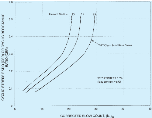
\left(q _ {\mathrm{CIN}}\right) _ {\mathrm{CS}} = k _ {\mathrm{C}} q _ {\mathrm{CIN}}

Chart

FIG. 28 RELATION BETWEEN CRR AND $(N_{1})_{60}$ FOR SAND FOR $M_{w}$ 7.5 EARTHQUAKES

where

$k_{c}$ = Correction factor to account for grain characteristics

\left| \begin{array}{l} = \left\{ \begin{array}{l} 1. 0 (\text {for} I _ {\mathrm{c}} \leq 1. 6 4) \\ - 0. 4 0 3 I _ {c} ^ {4} + 5. 5 8 1 I _ {c} ^ {3} - 2 1. 6 3 I _ {c} ^ {2} + \\ 3 3. 7 5 I _ {c} - 1 7. 8 8 \quad (\text {for} I _ {\mathrm{c}} > 1. 6 4), \text {and} \end{array} \right. \\ I _ {\mathrm{c}} = \sqrt {(3 . 4 7 - \log Q) ^ {2} + (1 . 2 2 - \log F) ^ {2}} \\ Q = \left(\frac {q _ {\mathrm{c}} - \sigma_ {\mathrm{vo}}}{P _ {\mathrm{a}}}\right) \left(\frac {P _ {\mathrm{a}}}{\sigma_ {\mathrm{vo}} ^ {\prime}}\right) ^ {\mathrm{n}} \\ F = 1 0 0 \left(\frac {f _ {\mathrm{s}}}{q _ {\mathrm{c}} - \sigma_ {\mathrm{vo}}}\right) \text {percent, and} \end{array} \right.

where $f_{\mathrm{s}} =$ measured sleeve friction.

Using $(q_{\mathrm{C1N}})_{\mathrm{CS}}$ find the value of $CRR_{7.5}$ using Fig. 29. Alternatively, the $CRR_{7.5}$ can be found using following equations:

C R R _ {7, 5} = \left\{ \begin{array}{l l} 0. 8 3 3 \left(\frac {\left(q _ {\mathrm{CIN}}\right) _ {\mathrm{CS}}}{1 0 0 0}\right) + 0. 0 5, & 0 < \left(q _ {\mathrm{CIN}}\right) _ {\mathrm{CS}} < 5 0 \\ 9 3 \left(\frac {\left(q _ {\mathrm{CIN}}\right) _ {\mathrm{CS}}}{1 0 0 0}\right) ^ {3} + 0. 0 8, & 5 0 \leq \left(q _ {\mathrm{CIN}}\right) _ {\mathrm{CS}} < 1 6 0 \end{array} \right.

6(c) Using shear wave velocity

Apply correction for overburden stress to shear wave velocity $V_{\mathrm{s}}$ for clean sands using:

V _ {\mathrm{s} 1} = \left(\frac {P _ {\mathrm{a}}}{\sigma_ {\mathrm{vo}} ^ {\prime}}\right) ^ {0. 2 5} V _ {\mathrm{s}}

where $(V_{\mathrm{s1}})$ is overburden stress corrected shear wave velocity. Using $V_{\mathrm{s1}}$ find the value of $CRR_{7.5}$ using Fig. 30. Alternatively, the $CRR_{7.5}$ can be found using following equation:

\left| C R R _ {7. 5} = a \left(\frac {V _ {\mathrm{s} 1}}{1 0 0}\right) ^ {2} + b \left(\frac {1}{V _ {\mathrm{s} 1} ^ {*} - V _ {\mathrm{s} 1}} - \frac {1}{V _ {\mathrm{s} 1} ^ {*}}\right) \right|

where $V_{\mathrm{s1}}^{*}$ is limiting upper value of $V_{\mathrm{s1}}$ for liquefaction occurrence; $a$ and $b$ are curve fitting parameters. The values of $a$ and $b$ in Fig. 30 are 0.022 and 2.8, respectively. $V_{\mathrm{s1}}^{*}$ can be assumed to vary linearly from $200~\mathrm{m / s}$ for soils with fine content of 35 percent, to 215 m/s for soils with fine contents of 5 percent or less.

Step 7 — Calculate the factor of safety FS against initial liquefaction using:

F S = \frac {C R R}{C S R},

where CSR is as estimated in Step 4 and CRR in Step 5. When the design ground motion is conservative, earthquake related permanent ground deformation is generally small, if $FS \geq 1.2$ .

Step 8 — If $FS < 1$ , then the soil is assumed to liquefy.

PART 6 STRUCTURAL DESIGN — SECTION 1 LOADS, FORCES AND EFFECTS

Chart

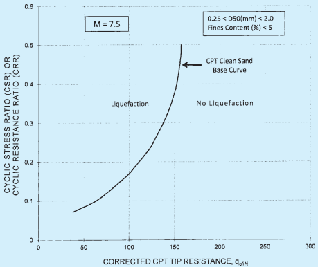
FIG. 29 RELATION BETWEEN $CRR$ AND $(q_{\mathrm{CIN}})_{\mathrm{cs}}$ FOR $M_w$ 7.5 EARTHQUAKES

Chart

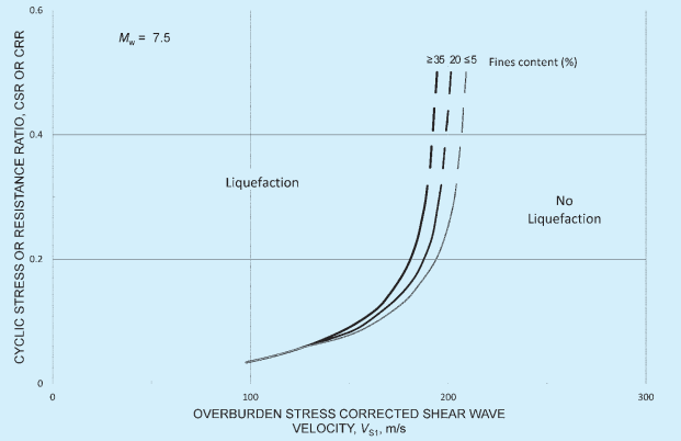
FIG. 30 RELATION BETWEEN CRR AND $V_{\mathrm{s1}}$ FOR $M_{\mathrm{w}}$ 7.5 EARTHQUAKES

Table 50Recommended Standardized SPT Equipment {see Accepted Standard [6-1(29)]} [Clause J-1, Step: 6(a)]

Sl No.	Element	Standard Specification
(1)	(2)	(3)
i)	Sampler	Standard split-spoon sampler with, Outside diameter, $OD = 51 \text{ mm}$ ; and Inside diameter, $ID = 35 \text{ mm}$ (constant, that is, no room for liners in the barrel).
ii)	Drill rods	$A \ or \ AW$ type for depths less than $15.2 \text{ m}$ ; $N \ or \ NW$ type for greater depths
iii)	Hammer	Standard (safety) hammer with,a) weight = 63.5 kg; andb) drop height = 762 mm (delivers 60 percent of theoretical free fall energy)
iv)	Rope	Two wraps of rope around the pulley
v)	Borehole	100-130 mm diameter rotary borehole with bentonite mud for borehole stability (hollow stem augers where SPT is taken through the stem)
vi)	Drill bit	Upward deflection of drilling mud (tricone or baffled drag bit)
vii)	Blow count rate	30 to 40 blows per minute
viii)	Penetration resistant count	Measured over range of 150 mm – 450 mm of penetration into the ground

Table 51Correction Factors for Non-Standard SPT Procedures and Equipment [Clause J-1, Step: 6(a)]

Sl No.	Correction for	Correction Factor
(1)	(2)	(3)
i)	Non-standard hammer type	$C_{\text{HT}} = \begin{cases} 0.75 & (\text{for Donut hammer with rope and pulley}) \\ 1.33 & (\text{for Donut hammer with trip/auto}) \end{cases}$ andEnergy ratio = 80 percent,
ii)	Non-standard hammer weight or height of fall	$C_{\text{HW}} = \frac{HW}{48\ 387}$ where $H = \text{height of fall (mm), and } W = \text{hammer weight (kg)}$
iii)	Non-standard sampler setup (standard samples with room for liners, but used without liners)	$C_{\text{ss}} = \begin{cases} 1.1 & (\text{for loose sand}) \\ 1.2 & (\text{for dense sand}) \end{cases}$
iv)	Non-standard sampler setup (standard samples with room forliners, but liners are used)	$C_{\text{ss}} = \begin{cases} 0.9 & (\text{for loose sand}) \\ 0.8 & (\text{for dense sand}) \end{cases}$
v)	Short rod length	$C_{\text{RL}} = 0.75$ (for rod length 0-3 m) $C_{\text{RL}} = 0.80$ (for rod length 3-4 m) $C_{\text{RL}} = 0.85$ (for rod length 4-6 m) $C_{\text{RL}} = 0.95$ (for rod length 6-10 m) $C_{\text{RL}} = 1.0$ (for rod length 10-30 m)
vi)	Non-standard borehole diameter	$C_{\text{BD}} = \begin{cases} 1.00 & (\text{for bore hole diameter of 65-115 mm}) \\ 1.05 & (\text{for bore hole diameter of 150 mm}) \\ 1.15 & (\text{for bore hole diameter of 200 mm}) \end{cases}$
NOTES
1 $N =$ Uncorrected SPT blow count.
2 $C_{60} = C_{\text{HT}} C_{\text{HW}} C_{\text{SS}} C_{\text{RL}} C_{\text{BD}}$
3 $N_{60} = NC_{60}$
4 $C_{\text{N}} =$ Correction factor for overburden pressure $(N_1)_{60} = C_{\text{N}} C_{60} N$ .

PART 6 STRUCTURAL DESIGN — SECTION 1 LOADS, FORCES AND EFFECTS

ANNEX K

(Clause 5.3.4.2)

LIST OF SOME IMPORTANT TOWNS AND THEIR SEISMIC ZONE FACTOR (Z)

Town	Zone	Z	Town	Zone	Z
Agra	III	0.16	Jhansi	II	0.10
Ahmedabad	III	0.16	Jodhpur	II	0.10
Ajmer	II	0.10	Jorhat	V	0.36
Allahabad	II	0.10	Kakrapara	III	0.16
Almora	IV	0.24	Kalpakkam	III	0.16
Ambala	IV	0.24	Kanchipuram	III	0.16
Amritsar	IV	0.24	Kanpur	III	0.16
Asansol	III	0.16	Karwar	III	0.16
Aurangabad	II	0.10	Kochi	III	0.16
Bahraich	IV	0.24	Kohima	V	0.36
Barauni	IV	0.24	Kolkata	III	0.16
Bareilly	III	0.16	Kota	II	0.10
Bathinda	III	0.16	Kurnool	II	0.10
Belgaum	III	0.16	Lucknow	III	0.16
Bengaluru	II	0.10	Ludhiana	IV	0.24
Bhilai	II	0.10	Madurai	II	0.10
Bhopal	II	0.10	Mandi	V	0.36
Bhubaneswar	III	0.16	Mangaluru	III	0.16
Bhuj	V	0.36	Mungher	IV	0.24
Bijapur	III	0.16	Moradabad	IV	0.24
Bikaner	III	0.16	Mumbai	III	0.16
Bokaro	III	0.16	Mysuru	II	0.10
Bulandshahr	IV	0.24	Nagpur	II	0.10
Burdwan	III	0.16	Nagarjunasagar	II	0.10
Calicut (Kozhikode)	III	0.16	Nainital	IV	0.24
Chandigarh	IV	0.24	Nashik	III	0.16
Chennai	III	0.16	Nellore	III	0.16
Chitradurga	II	0.10	Osmanabad	III	0.16
Coimbatore	III	0.16	Panjim	III	0.16
Cuddalore	II	0.10	Patiala	III	0.16
Cuttack	III	0.16	Patna	IV	0.24
Darbhanga	V	0.36	Pilibhit	IV	0.24
Darjeeling	IV	0.24	Pondicherry (Puducherry)	II	0.10
Dharwad	III	0.16	Pune	III	0.16
Dehra Dun	IV	0.24	Raipur	II	0.10
Dharampuri	III	0.16	Rajkot	III	0.16
Delhi	IV	0.24	Ranchi	II	0.10
Durgapur	III	0.16	Roorkee	IV	0.24
Gangtok	IV	0.24	Rourkela	II	0.10
Guwahati	V	0.36	Sadiya	V	0.36
Gulbarga	II	0.10	Salem	III	0.16
Gaya	III	0.16	Shillong	V	0.36
Gorakhpur	IV	0.24	Shimla	IV	0.24
Hyderabad	II	0.10	Sironj	II	0.10
Imphal	V	0.36	Solapur	III	0.16
Jabalpur	III	0.16	Srinagar	V	0.36
Jaipur	II	0.10	Surat	III	0.16
Jamshedpur	II	0.10	Tarapur	III	0.16

Town	Zone	Z
Tezpur	V	0.36
Thane	III	0.16
Thanjavur	II	0.10
Thiruvananthapuram	III	0.16
Tiruchirappalli	II	0.10
Tiruvannamalai	III	0.16

Town	Zone	Z
Udaipur	II	0.10
Vadodara	III	0.16
Varanasi	III	0.16
Vellore	III	0.16
Vijayawada	III	0.16
Vishakhapatnam	II	0.10